Semantic Segmentation Using Deep Learning

Project Description

This project involved the creation of a convolutional neural network with a Unet architecture for the identification of drone racing gates. The network was trained and tested on a dataset artificially generated from Blender and augmented using Python’s torchvision.transforms library. Additionally, the network reached an accuracy of 95% on the testing sample and demonstrated success at tracking gates in a sample video that was not a part of the dataset.

Methodology

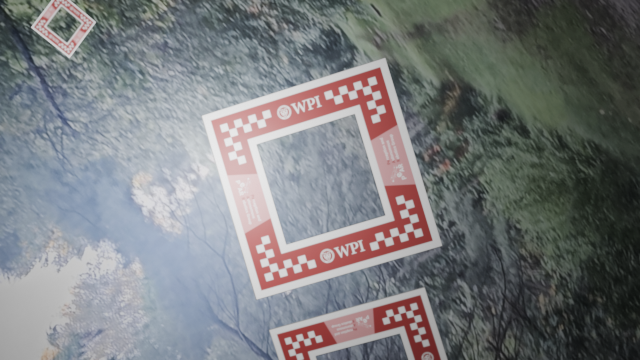
Our team used a rendering software called Blender to generate 3D scenes. Blender contains a built-in Python interpreter and API, allowing users to write scripts to manipulate and export scenes. We set up a scene with multiple windows on a black background. Our image generation script would randomly move windows, import backgrounds, adjust lighting, and change the camera position within the scene five thousand times, exporting the scene to an image after each iteration.

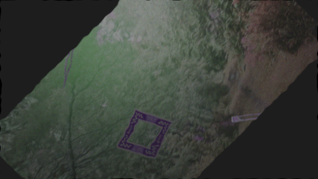
We created an image augmentation script to import the images and apply various transformations onto them, expanding our dataset size to fifty thousand images. Transformations included rotation, resizing, blurring, adding noise, adding color jitter, inversion, and simulating the image being put under water.

We decided to use the U-Net architecture for our model, which consists of an encoder to extract image features and a decoder to create a mask out of these features. In our specific case, the model should predict the location of the windows in an image. The output labels were a mask of the original image, where the window targets are white and the rest of the image is black, as seen above.

With U-Net's encoder-decoder architecture, we have four encoder steps, four decoder steps, and a bottom step linking the two. These steps consist of a small pattern that repeats twice, as well as either an Upsample or MaxPool2D step. This pattern consists of convolution layer (which was padded so that it did not change the size of the image), a batch normalization layer to normalize the inputs, and a ReLU activation layer (which converts all negative input values to zero but keeps other input values the same). The batch normalization layers prevent the input values from being too big, preventing the output from growing to infinity.

Each encoder layer splits up the image into smaller pieces, the first of which are usually called feature layers. Each encoder layer is the pattern we described earlier, twice, followed by a MaxPool2D step. The MaxPool2D layer is what actually decreases the image size, using (in our case), a kernel size of 5, a stride of 2, and a padding of 2. During our encoder steps, we gradually decrease the size of our kernel, starting at 11, then decreasing to 7, 5, and finally 3, where it remains for the rest of our Conv2d layers.

Each decoder layer combines these features back into a larger image. Each decoder step is an Upsample layer, which actually does the combining, followed by the same pattern mentioned twice already. Separating the encoder+decoder layers is a bottom step, which is just the same pattern we've mentioned thrice.

Most U-Net architectures contain skip connections, which preserve the outputs of previous encoder layers and add them to the corresponding decoder layers, thereby preventing the gradients from reaching zero and freezing progress within the neural network. We initially wrote our network intending to add skip connections later, but when we trained our network, we found that its accuracy was sufficient. Given the amount of time to retrain our models, we decided to forgo the skip connections and stick with our current structure.

In training this model, we utilized Binary Cross Entropy Loss (BCELoss), which uses the log of the model output, along with the label, to determine the loss. BCELoss is a common solution for binary classification, which matches our use case. For training, we utilized ADAM with a learning rate of 1e^-4.

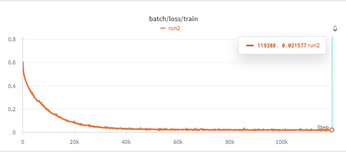
We trained with batches of eight images for 24 hours, totaling around 433,000 batches and 69 epochs. At around 100,000 batches and 15 epochs, our model settled around a 5% training loss, only improving to 4% in subsequent batches. However, at this step we realized that within our dataset, we made the windows too small, such that it did not accurately reflect the video we were to test against. We needed to regenerate our 5k renders from Blender with a larger scale for the windows, then retrain for another 8 hours, totalling 140,000 batches and 21 epochs. We processed the final video using the model after 21 epochs, at a loss of 12.0% (or 88.0% accuracy). We also tested with partially trained models, using epoch 3 (38.5% loss) and epoch 13 (12.8% loss) for comparison, but the later model was either equal or better on every frame, so we kept the newer model. A video of this comparison can be seen above.

The model's training loss progression can be seen above. At the beginning, the model improves drastically, but once it hits about 40k batches (only 6 epochs), the model barely improves at all. By batch 100k (epoch 15), the validation loss had only improved 9%, from 23% loss at batch 40k to a 14% loss at 100k.

After retraining our model to perform better, it did quite well on the final video. However, we once again did not account for exactly how large the window gets in the video, and it once again was not reflected properly in the dataset. As such, that part of the video is lacking in clarity compared to the rest.

Reflection

Overall, this process taught us valuable skills in image generation, dataset augmentation, and implementing more sophisticated machine learning architectures. One mistake we made that we would do differently next time, was not checking the video before generating our dataset. In the final video that we tested our dataset against, the windows were much closer, took up much more of the screen, and were sometimes cut off by the edge of the frame. In contrast, the dataset we trained our algorithm on had much smaller windows, often showcased these windows at a much sharper angle, and rarely had windows that were cut off by the edge of the frame. If we had accounted for these attributes in our dataset, we may have had more success when testing it. Despite this, we were still able to achieve an accuracy of 88.0% for our test dataset and adequately track the frames in the test video.